Complicated H-alpha Line Fitting
"""
Example demonstrating how to fit a complex H-alpha profile after
subtracting off a satellite line (in this case, He I 6678.151704)
"""
import pyspeckit

sp = pyspeckit.Spectrum('sn2009ip_halpha.fits')

# start by plotting a small region around the H-alpha line
sp.plotter(xmin=6100,xmax=7000,ymax=2.23,ymin=0)

# the baseline (continuum) fit will be 2nd order, and excludes "bad"
# parts of the spectrum
# The exclusion zone was selected interactively
# (i.e., cursor hovering over the spectrum)
sp.baseline(xmin=6100, xmax=7000,
        exclude=[6450,6746,6815,6884,7003,7126,7506,7674,8142,8231],
        subtract=False, reset_selection=True, highlight_fitregion=True,
        order=2)

# Fit a 4-parameter voigt (figured out through a series if guess and check fits)
sp.specfit(guesses=[2.4007096541802202,  6563.2307968382256, 3.5653446153950314,  1,
                    0.53985149324131965, 6564.3460908526877, 19.443226155616617,  1,
                    0.11957267912208754, 6678.3853431367716, 4.1892742162283181,  1,
                    0.10506431180136294, 6589.9310414408683, 72.378997529374672,  1,],
                    fittype='voigt')

# Now overplot the fitted components with an offset so we can see them
# the add_baseline=True bit means that each component will be displayed
# with the "Continuum" added
# If this was off, the components would be displayed at y=0
# the component_yoffset is the offset to add to the continuum for plotting
# only (a constant)
sp.specfit.plot_components(add_baseline=True,component_yoffset=-0.2)

# Now overplot the residuals on the same graph by specifying which axis to overplot it on
# clear=False is needed to keep the original fitted plot drawn
# yoffset is the offset from y=zero
sp.specfit.plotresiduals(axis=sp.plotter.axis,clear=False,yoffset=0.20,label=False)

# save the figure
sp.plotter.savefig("SN2009ip_UT121002_Halpha_voigt_zoom.png")

# print the fit results in table form
# This includes getting the equivalent width for each component using sp.specfit.EQW
print(" ".join(["%15s %15s" % (s,s+"err") for s in sp.specfit.parinfo.parnames]),
" ".join(["%15s" % ("EQW"+str(i)) for i,w in enumerate(sp.specfit.EQW(components=True))]))
print(" ".join(["%15g %15g" % (par.value,par.error) for par in sp.specfit.parinfo]),
" ".join(["%15g" % w for w in sp.specfit.EQW(components=True)]))
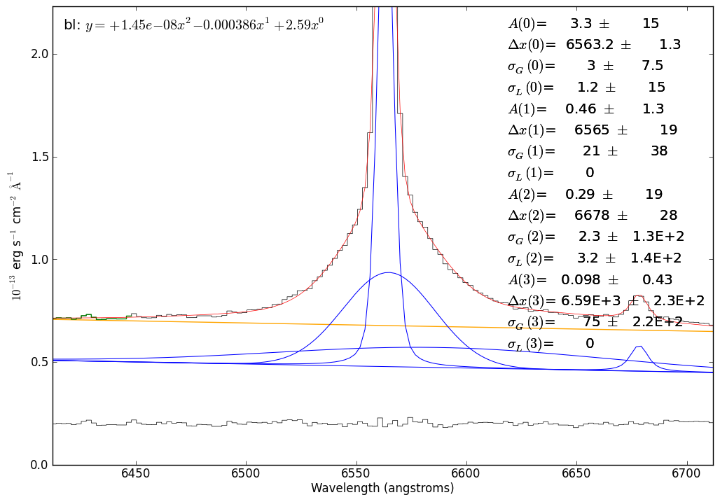
# zoom in further for a detailed view of the profile fit
sp.plotter.axis.set_xlim(6562-150,6562+150)
sp.plotter.savefig("SN2009ip_UT121002_Halpha_voigt_zoomzoom.png")
# now we'll re-do the fit with the He I line subtracted off
# first, create a copy of the spectrum
just_halpha = sp.copy()
# Second, subtract off the model fit for the He I component
# (identify it by looking at the fitted central wavelengths)
just_halpha.data -= sp.specfit.modelcomponents[2,:]
# re-plot
just_halpha.plotter(xmin=6100,xmax=7000,ymax=2.00,ymin=-0.3)
# this time, subtract off the baseline - we're now confident that the continuum
# fit is good enough
just_halpha.baseline(xmin=6100, xmax=7000,
exclude=[6450,6746,6815,6884,7003,7126,7506,7674,8142,8231],
subtract=True, reset_selection=True, highlight_fitregion=True, order=2)
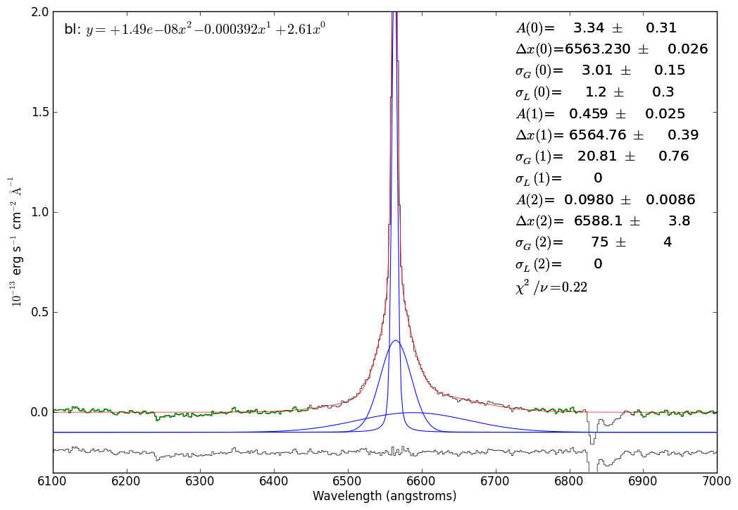
# Do a 3-component fit now that the Helium line is gone
# I've added some limits here because I know what parameters I expect of my fitted line
just_halpha.specfit(guesses=[2.4007096541802202, 6563.2307968382256, 3.5653446153950314, 1,
0.53985149324131965, 6564.3460908526877, 19.443226155616617, 1,
0.10506431180136294, 6589.9310414408683, 50.378997529374672, 1,],
fittype='voigt',
xmin=6100,xmax=7000,
limitedmax=[False,False,True,True]*3,
limitedmin=[True,False,True,True]*3,
limits=[(0,0),(0,0),(0,100),(0,100)]*3)
# overplot the components and residuals again
just_halpha.specfit.plot_components(add_baseline=False,component_yoffset=-0.1)
just_halpha.specfit.plotresiduals(axis=just_halpha.plotter.axis,
clear=False, yoffset=-0.20, label=False)
# The "optimal chi^2" isn't a real statistical concept, it's something I made up
# However, I think it makes sense (but post an issue if you disagree!):
# It uses the fitted model to find all pixels that are above the noise in the spectrum
# then computes chi^2/n using only those pixels
just_halpha.specfit.annotate(chi2='optimal')
# save the figure
just_halpha.plotter.savefig("SN2009ip_UT121002_Halpha_voigt_threecomp.png")
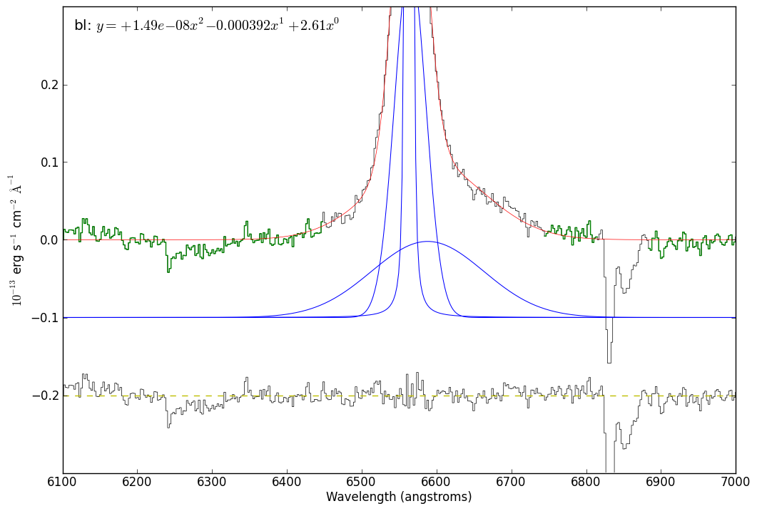
# A new zoom-in figure
import pylab
# now hide the legend
just_halpha.specfit.fitleg.set_visible(False)
# overplot a y=0 line through the residuals (for reference)
pylab.plot([6100,7000],[-0.2,-0.2],'y--')
# zoom vertically
pylab.gca().set_ylim(-0.3,0.3)
# redraw & save
pylab.draw()
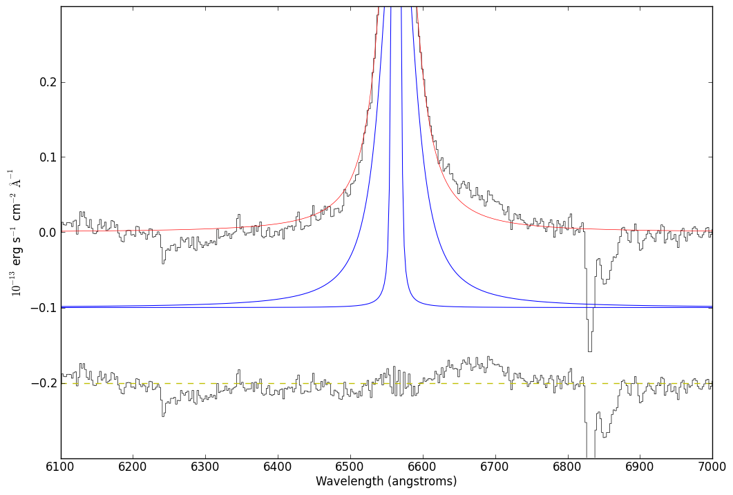
just_halpha.plotter.savefig("SN2009ip_UT121002_Halpha_voigt_threecomp_zoom.png")
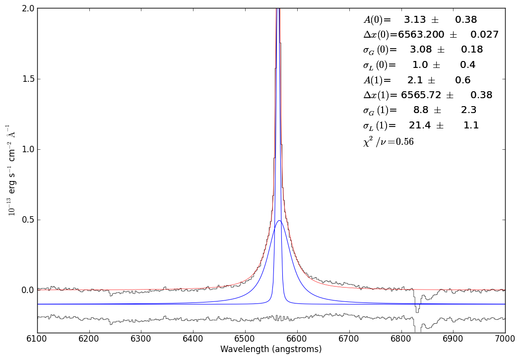
# Part of the reason for doing the above work is to demonstrate that a
# 3-component fit is better than a 2-component fit
#
# So, now we do the same as above with a 2-component fit

just_halpha.plotter(xmin=6100,xmax=7000,ymax=2.00,ymin=-0.3)
just_halpha.specfit(guesses=[2.4007096541802202, 6563.2307968382256, 3.5653446153950314, 1,
                    0.53985149324131965, 6564.3460908526877, 19.443226155616617,  1],
                    fittype='voigt')
just_halpha.specfit.plot_components(add_baseline=False,component_yoffset=-0.1)
just_halpha.specfit.plotresiduals(axis=just_halpha.plotter.axis,
                                  clear=False, yoffset=-0.20,label=False)
just_halpha.specfit.annotate(chi2='optimal')
just_halpha.plotter.savefig("SN2009ip_UT121002_Halpha_voigt_twocomp.png")
just_halpha.specfit.fitleg.set_visible(False)
pylab.plot([6100,7000],[-0.2,-0.2],'y--')
pylab.gca().set_ylim(-0.3,0.3)
pylab.draw()
just_halpha.plotter.savefig("SN2009ip_UT121002_Halpha_voigt_twocomp_zoom.png")