LTE Line Model example: Line identification

import numpy as np

# retrieve the data
import requests

# 10 MB file: stream it, but it should be able to load in memory
response = requests.get('https://dataverse.harvard.edu/api/access/datafile/:persistentId?persistentId=doi:10.7910/DVN/8QJT3K/POCX2W', stream=True)

with open('temp_cube.fits', 'wb') as fh:
    fh.write(response.content)

from spectral_cube import SpectralCube 
from astropy import units as u
# there is some junk at low frequency
cube = SpectralCube.read('temp_cube.fits').spectral_slab(218.14*u.GHz, 218.54*u.GHz)

# this isn't really right b/c of beam issues, but it's Good Enough
meanspec = cube.mean(axis=(1,2))
# have to hack this, which is _awful_ and we need to fix it
meanspec_K = meanspec.value * cube.beam.jtok(cube.spectral_axis)

import pyspeckit

sp = pyspeckit.Spectrum(xarr=cube.spectral_axis, data=meanspec_K)



# The LTE model doesn't include an explicit filling factor, so we impose one
fillingfactor = 0.05

# there's continuum in our spectrum, but it's also not modeled
offset = np.nanpercentile(sp.data.filled(np.nan), 20)

# look at a couple species
# Be cautious! Not all line catalogs have all of these species, some species
# can result in multiple matches from splatalogue, and definitely not all
# species have the same column and excitation
species_list = ('CH3OH', 'HCCCN', 'H2CO', 'CH3OCHO', 'CH3OCH3', 'C2H5CN',)
# 'C2H3CN' is pretty definitely not here at the constant assumed column

# make a set of subplots:
import pylab as pl
fig, axes = pl.subplots(len(species_list)+1, 1, figsize=(18,14), num=1)
pl.draw()

from pyspeckit.spectrum.models import lte_molecule
mods = []
for species, axis in zip(species_list, axes):
    # search for lines within +/- 0.5 GHz of the min/max (to account for velocity offset, generously)
    freqs, aij, deg, EU, partfunc = lte_molecule.get_molecular_parameters(species,
                                                                          fmin=sp.xarr.min()-0.5*u.GHz,
                                                                          fmax=sp.xarr.max()+0.5*u.GHz)

    mod = lte_molecule.generate_model(xarr=sp.xarr, vcen=50*u.km/u.s,
                                      width=3*u.km/u.s, tex=100*u.K,
                                      column=1e17*u.cm**-2, freqs=freqs,
                                      aij=aij, deg=deg, EU=EU,
                                      partfunc=partfunc)
    mods.append(mod)

    sp.plotter(axis=axis, figure=fig, clear=False)
    sp.plotter.axis.plot(sp.xarr, mod*fillingfactor+offset, label=species, zorder=-1)
    sp.plotter.axis.text(0.5,0.9,species,transform=axis.transAxes)

    if axis != axes[-1]:
        axis.set_xlabel("")
        axis.set_xticklabels([])
    if axis != axes[len(species_list) // 2]:
        axis.set_ylabel("")


axis = axes[-1]
sp.plotter(axis=axis, figure=fig, clear=False)
sp.plotter.axis.plot(sp.xarr, np.nansum(mods,axis=0)*fillingfactor+offset, label='Sum', zorder=-1)
sp.plotter.axis.text(0.5,0.9,'Sum',transform=axis.transAxes)

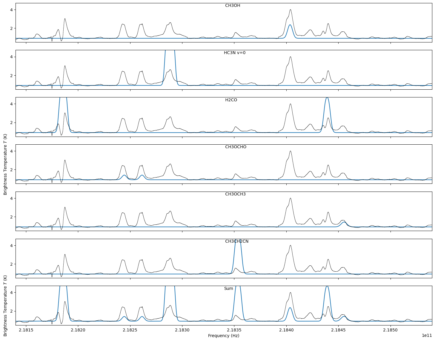
W51 spectrum with LTE lines at T_X = 100, N=10^17

[edit this page on github]

[edit this page on bitbucket]