Monte Carlo examples
There are (at least) two packages implementing Monte Carlo sampling available
in python: pymc and emcee. pyspeckit includes interfaces to both. With
the pymc interface, it is possible to define priors that strictly limit the
parameter space. So far that is not possible with emcee.
The examples below use a custom plotting package from agpy. It is a relatively simple but convenient wrapper around numpy’s histogram2d. pymc_plotting takes care of indexing, percentile determination, and coloring.
The example below shows the results of a gaussian fit to noisy data (S/N ~ 6).
The parameter space is then explored with pymc and emcee in order to examine
the correlation between width and amplitude.
import pyspeckit
import numpy as np

# Create our own gaussian centered at 0 with width 1, amplitude 5, and
# gaussian noise with amplitude 1
x = pyspeckit.units.SpectroscopicAxis(np.linspace(-10,10,50), unit='km/s')
e = np.random.randn(50)
d = np.exp(-np.asarray(x)**2/2.)*5 + e

# create the spectrum object
sp = pyspeckit.Spectrum(data=d, xarr=x, error=np.ones(50)*e.std())
# fit it
sp.specfit(fittype='gaussian', guesses=[1,0,1])
# then get the pymc values
MCuninformed = sp.specfit.get_pymc()
MCwithpriors = sp.specfit.get_pymc(use_fitted_values=True)
MCuninformed.sample(101000,burn=1000,tune_interval=250)
MCwithpriors.sample(101000,burn=1000,tune_interval=250)

# MC vs least squares:
print(sp.specfit.parinfo)
# Param #0   AMPLITUDE0 =         4.51708 +/-        0.697514
# Param #1       SHIFT0 =       0.0730243 +/-        0.147537
# Param #2       WIDTH0 =        0.846578 +/-        0.147537   Range:   [0,inf)


print(MCuninformed.stats()['AMPLITUDE0'],MCuninformed.stats()['WIDTH0'])
#  {'95% HPD interval': array([ 2.9593463 ,  5.65258618]),
#   'mc error': 0.0069093803546614969,
#   'mean': 4.2742994714387068,
#   'n': 100000,
#   'quantiles': {2.5: 2.9772782318342288,
#    25: 3.8023115438555615,
#    50: 4.2534542126311479,
#    75: 4.7307441549353229,
#    97.5: 5.6795448148793293},
#   'standard deviation': 0.68803712503362213},
#  {'95% HPD interval': array([ 0.55673242,  1.13494423]),
#   'mc error': 0.0015457954546501554,
#   'mean': 0.83858499779600593,
#   'n': 100000,
#   'quantiles': {2.5: 0.58307734425381375,
#    25: 0.735072721596429,
#    50: 0.824695077252244,
#    75: 0.92485225882530664,
#    97.5: 1.1737067304111048},
#   'standard deviation': 0.14960171537498618}


print(MCwithpriors.stats()['AMPLITUDE0'],MCwithpriors.stats()['WIDTH0'])
#  {'95% HPD interval': array([ 3.45622857,  5.28802497]),
#   'mc error': 0.0034676818027776788,
#   'mean': 4.3735547007147595,
#   'n': 100000,
#   'quantiles': {2.5: 3.4620369729291913,
#    25: 4.0562790782065052,
#    50: 4.3706408236777481,
#    75: 4.6842793868186332,
#    97.5: 5.2975444315549947},
#   'standard deviation': 0.46870135068815683},
#  {'95% HPD interval': array([ 0.63259418,  1.00028015]),
#   'mc error': 0.00077504289680683364,
#   'mean': 0.81025043433745358,
#   'n': 100000,
#   'quantiles': {2.5: 0.63457050661326331,
#    25: 0.7465422649464849,
#    50: 0.80661741451336577,
#    75: 0.87067288601310233,
#    97.5: 1.0040591994661381},
#   'standard deviation': 0.093979950317277294}


# optional
from mpl_plot_templates import pymc_plotting
import pylab
pymc_plotting.hist2d(MCuninformed,'AMPLITUDE0','WIDTH0',clear=True,bins=[25,25])
pymc_plotting.hist2d(MCwithpriors,'AMPLITUDE0','WIDTH0',contourcmd=pylab.contour,colors=[(0,1,0,1),(0,0.5,0.5,1),(0,0.75,0.75,1),(0,1,1,1),(0,0,1,1)],clear=False,bins=[25,25])
pylab.plot([5],[1],'k+',markersize=25, zorder=1000)
pylab.savefig("pymc_example_Gaussian_amplitude_vs_width.pdf")

# Now do the same with emcee
emcee_ensemble = sp.specfit.get_emcee()
p0 = emcee_ensemble.p0 * (np.random.randn(*emcee_ensemble.p0.shape) / 10. + 1.0)
pos,logprob,state = emcee_ensemble.run_mcmc(p0,100000)

plotdict = {'AMPLITUDE0':emcee_ensemble.chain[:,:,0].ravel(),
            'WIDTH0':emcee_ensemble.chain[:,:,2].ravel()}
pymc_plotting.hist2d(plotdict,'AMPLITUDE0','WIDTH0',fignum=2,bins=[25,25],clear=True)
pylab.plot([5],[1],'k+',markersize=25)
pylab.savefig("emcee_example_Gaussian_amplitude_vs_width.pdf")
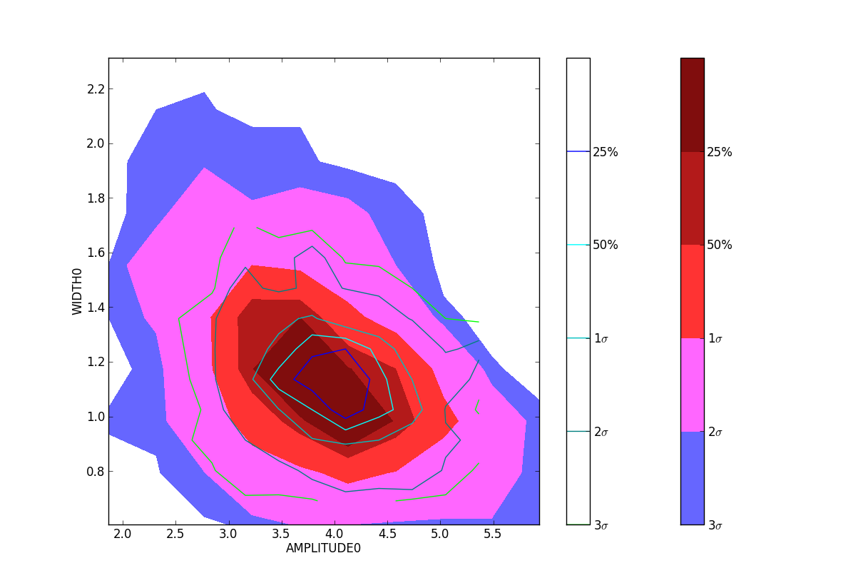
The Amplitude-Width parameter space sampled by pymc with (lines) and without (solid) priors. There is moderate anticorrelation between the line width and the peak amplitude. The + symbol indicates the input parameters; the model does a somewhat poor job of recovering the true values (in case you’re curious, there is no intrinsic bias - if you repeat the above fitting procedure a few hundred times, the mean fitted amplitude is 5.0).
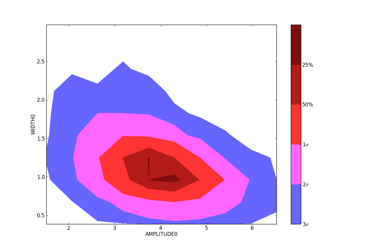
The parameter space sampled with emcee and binned onto a 25x25 grid. Note
that emcee has 6x as many points (and takes about 6x as long to run) because
there are 6 “walkers” for the 3 parameters being fit.