Radio Fitting: HCN example with freely varying hyperfine amplitudes
Example hyperfine line fitting for the HCN 1-0 line.
from __future__ import print_function
import pyspeckit
import pylab as pl
import astropy.units as u

# Load the spectrum & properly identify the units
# The data is from http://adsabs.harvard.edu/abs/1999A%26A...348..600P
sp = pyspeckit.Spectrum('02232_plus_6138.txt')
sp.xarr.set_unit(u.km/u.s)
sp.xarr.refX = 88.63184666e9 * u.Hz
sp.xarr.velocity_convention = 'radio'
sp.xarr.xtype='velocity'
sp.unit='$T_A^*$'

# set the error array based on a signal-free part of the spectrum
sp.error[:] = sp.stats((-35,-25))['std']
# Register the fitter
# The HCN fitter is 'built-in' but is not registered by default; this example
# shows how to register a fitting procedure
# 'multi' indicates that it is possible to fit multiple components and a
# background will not automatically be fit
# 5 is the number of parameters in the model (line center,
# line width, and amplitude for the 0-1, 2-1, and 1-1 lines)
sp.Registry.add_fitter('hcn_varyhf',pyspeckit.models.hcn.hcn_varyhf_amp_fitter,5)

# This one is the same, but with fixed relative ampltidue hyperfine components
sp.Registry.add_fitter('hcn_fixedhf',pyspeckit.models.hcn.hcn_amp,3)

# Plot the results
sp.plotter()
# Run the fixed-ampltiude fitter and show the individual fit components
sp.specfit(fittype='hcn_fixedhf',
           multifit=None,
           guesses=[1,-48,0.6],
           show_hyperfine_components=True)
# Now plot the residuals offset below the original
sp.specfit.plotresiduals(axis=sp.plotter.axis,clear=False,yoffset=-1,color='g',label=False)
sp.plotter.reset_limits(ymin=-2)

# Save the figure (this step is just so that an image can be included on the web page)
sp.plotter.savefig('hcn_fixedhf_fit.png')

# Run the variable-ampltiude fitter and show the individual fit components
# Note the different order of the arguments (velocity, width, then three amplitudes)
sp.specfit(fittype='hcn_varyhf',
           multifit=None,
           guesses=[-48,1,0.2,0.6,0.3],
           show_hyperfine_components=True,
           clear=True)

# Again plot the residuals
sp.specfit.plotresiduals(axis=sp.plotter.axis,clear=False,yoffset=-1,color='g',label=False)
sp.plotter.reset_limits(ymin=-2)

# Save the figure
sp.plotter.savefig('hcn_freehf_fit.png')


# now do the same thing, but allow the widths to vary too
# there are 7 parameters:
# 1. the centroid
# 2,3,4 - the amplitudes of the 0-1, 2-1, and 1-1 lines
# 5,6,7 - the widths of the 0-1, 2-1, and 1-1 lines
sp.Registry.add_fitter('hcn_varyhf_width',pyspeckit.models.hcn.hcn_varyhf_amp_width_fitter,7)

# Run the fitter
sp.specfit(fittype='hcn_varyhf_width',
           multifit=None,
           guesses=[-48,0.2,0.6,0.3,1,1,1],
           show_hyperfine_components=True,
           clear=True)

# print the fitted parameters:
print(sp.specfit.parinfo)
# Param #0      CENTER0 =      -51.865 +/-       0.0525058
# Param #1    AMP10-010 =      1.83238 +/-       0.0773993   Range:   [0,inf)
# Param #2    AMP12-010 =      5.26566 +/-       0.0835981   Range:   [0,inf)
# Param #3    AMP11-010 =      3.02621 +/-       0.0909095   Range:   [0,inf)
# Param #4  WIDTH10-010 =      2.16711 +/-        0.118651   Range:   [0,inf)
# Param #5  WIDTH12-010 =      1.90987 +/-       0.0476163   Range:   [0,inf)
# Param #6  WIDTH11-010 =      1.64409 +/-        0.076998   Range:   [0,inf)

sp.specfit.plotresiduals(axis=sp.plotter.axis,clear=False,yoffset=-1,color='g',label=False)
sp.plotter.reset_limits(ymin=-2)

# Save the figure (this step is just so that an image can be included on the web page)
sp.plotter.savefig('hcn_freehf_ampandwidth_fit.png')

# Finally, how well does a 2-component fit work?
sp.specfit(fittype='hcn_fixedhf',
           multifit=None,
           guesses=[1,-48,0.6,0.1,-46,0.6],
           show_hyperfine_components=True,
           clear=True)
sp.specfit.plotresiduals(axis=sp.plotter.axis,clear=False,yoffset=-1,color='g',label=False)
sp.plotter.reset_limits(ymin=-2)

# Save the figure (this step is just so that an image can be included on the web page)
sp.plotter.savefig('hcn_fixedhf_fit_2components.png')
The green lines in the following figures all show the residuals to the fit
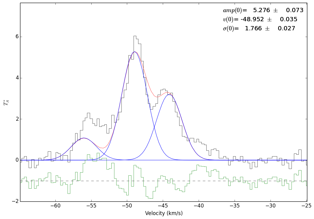
Fit to the 3 hyperfine components of HCN 1-0 simultaneously with fixed amplitudes. The (0)’s indicate that this is the 0’th velocity component being fit (though that velocity corresponds to the 12-01 component of the line)
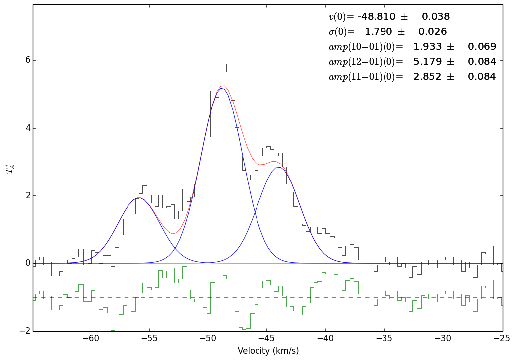
Fit to the 3 hyperfine components of HCN 1-0 simultaneously with freely varying amplitudes. The (0)’s indicate that this is the 0’th velocity component being fit
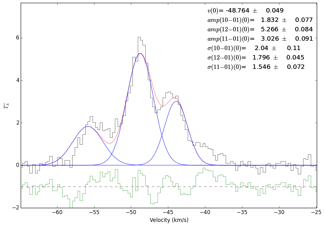
Fit to the 3 hyperfine components of HCN 1-0 simultaneously. The widths are allowed to vary in this example.
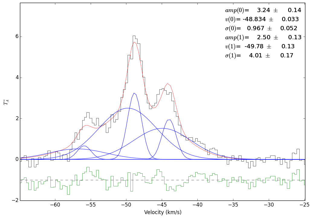
A two-component fit to the same spectrum. It appears to be a much better fit, hinting that there are indeed two components (though the fit is probably not unique)