Basic Plotting Guide

The plotting tool in pyspeckit is intended to make publication-quality plots straightforward to produce.

For details on the various plotting tools, please see the examples and the plotter documentation.

A few basic examples are shown in the snippet below, with comments describing the various steps. This example (https://github.com/jmangum/spectrumplot) shows how to use pyspeckit with spectral_cube to extract and label spectra. Other examples:

import numpy as np
from astropy import units as u
import pyspeckit

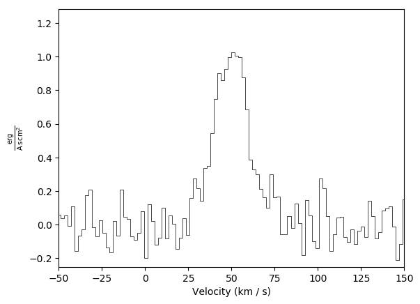
xaxis = np.linspace(-50,150,100.) * u.km/u.s
sigma = 10. * u.km/u.s
center = 50. * u.km/u.s
synth_data = np.exp(-(xaxis-center)**2/(sigma**2 * 2.))

# Add noise
stddev = 0.1
noise = np.random.randn(xaxis.size)*stddev
error = stddev*np.ones_like(synth_data)
data = noise+synth_data

# this will give a "blank header" warning, which is fine
sp = pyspeckit.Spectrum(data=data, error=error, xarr=xaxis,
                        unit=u.erg/u.s/u.cm**2/u.AA)

sp.plotter()
sp.plotter.savefig('basic_plot_example.png')

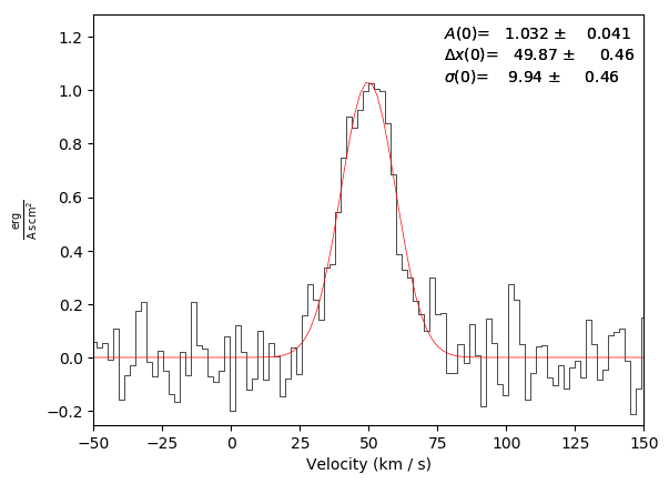
# Fit with automatic guesses
sp.specfit(fittype='gaussian')
# (this will produce a plot overlay showing the fit curve and values)
sp.plotter.savefig('basic_plot_example_withfit.png')

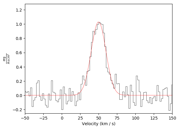
# Redo the overlay with no annotation

# remove both the legend and the model overlay
sp.specfit.clear()
# then re-plot the model without an annotation (legend)
sp.specfit.plot_fit(annotate=False)
sp.plotter.savefig('basic_plot_example_withfit_no_annotation.png')


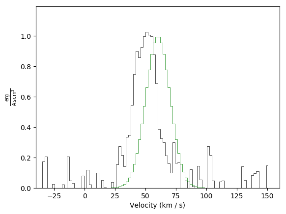
# overlay another spectrum
# We use the 'synthetic' spectrum with no noise, then shift it by 10 km/s
sp2 = pyspeckit.Spectrum(data=synth_data, error=None, xarr=xaxis+10*u.km/u.s,
                         unit=u.erg/u.s/u.cm**2/u.AA)

# again, remove the overlaid model fit
sp.specfit.clear()

# to overplot, you need to tell the plotter which matplotlib axis to use and
# tell it not to clear the plot first
sp2.plotter(axis=sp.plotter.axis,
            clear=False,
            color='g')

# sp2.plotter and sp.plotter can both be used here (they refer to the same axis
# and figure now)
sp.plotter.savefig('basic_plot_example_with_second_spectrum_overlaid_in_green.png')

# the plot window will follow the last plotted spectrum's limits by default;
# that can be overridden with the xmin/xmax keywords
sp2.plotter(axis=sp.plotter.axis,
            xmin=-100, xmax=200,
            ymin=-0.5, ymax=1.5,
            clear=False,
            color='g')
sp.plotter.savefig('basic_plot_example_with_second_spectrum_overlaid_in_green_wider_limits.png')


# you can also offset the spectra and set different 
# this time, we need to clear the axis first, then do a fresh overlay

# fresh plot
sp.plotter(clear=True)

# overlay, shifted down by 0.2 in y and with a wider linewidth
sp2.plotter(axis=sp.plotter.axis,
            offset=-0.2,
            clear=False,
            color='r',
            linewidth=2,
            alpha=0.5,
           )
# you can also modify the axis properties directly
sp.plotter.axis.set_ylim(-0.25, 1.1)
sp2.plotter.savefig('basic_plot_example_with_second_spectrum_offset_overlaid_in_red.png')

Basic plot example:

Basic plot example with a fit and an annotation (annotation is on by default):

Basic plot example with a fit, but with no annotation:

Basic plot example with a second spectrum overlaid in green:

Basic plot example with a second spectrum overlaid in green plus adjusted limits:

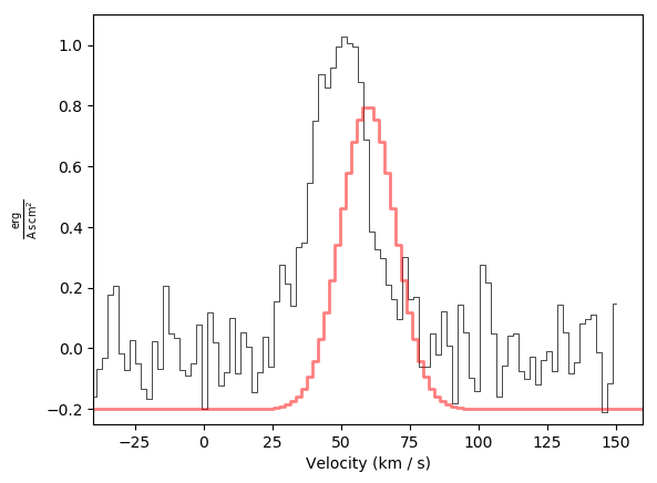
Basic plot example with a second spectrum offset and overlaid in red, again with adjusted limits:

API Documentation for Plotting

We include the API documentation for the generic model and fitter wrappers here.

class pyspeckit.spectrum.plotters.BoundMethodProxy(meth, callback=None)

class pyspeckit.spectrum.plotters.Plotter(Spectrum, autorefresh=True, title='', xlabel=None, silent=True, plotscale=1.0, **kwargs)

Class to plot a spectrum

activate_interactive_baseline_fitter(**kwargs)

Attempt to activate the interactive baseline fitter

activate_interactive_fitter()

Attempt to activate the interactive fitter

connect()

Connect to the matplotlib key-parsing interactivity

copy(parent=None)

Create a copy of the plotter with blank (uninitialized) axis & figure

[ parent ]

A spectroscopic axis instance that is the parent of the specfit instance. This needs to be specified at some point, but defaults to None to prevent overwriting a previous plot.

disconnect()

Disconnect the matplotlib interactivity of this pyspeckit plotter.

label(title=None, xlabel=None, ylabel=None, verbose_label=False, **kwargs)

Label the plot, with an attempt to parse standard units into nice latex labels

Parameters

title : str

xlabel : str

ylabel : str

verbose_label: bool :

line_ids(line_names, line_xvals, xval_units=None, auto_yloc=True, velocity_offset=None, velocity_convention='radio', auto_yloc_fraction=0.9, **kwargs)

Add line ID labels to a plot using lineid_plot http://oneau.wordpress.com/2011/10/01/line-id-plot/ https://github.com/phn/lineid_plot http://packages.python.org/lineid_plot/

Parameters

line_names : list

A list of strings to label the specified x-axis values

line_xvals : list

List of x-axis values (e.g., wavelengths) at which to label the lines. Can be a list of quantities.

xval_units : string

The unit of the line_xvals if they are not given as quantities

velocity_offset : quantity

A velocity offset to apply to the inputs if they are in frequency or wavelength units

velocity_convention : ‘radio’ or ‘optical’ or ‘doppler’

Used if the velocity offset is given

auto_yloc : bool

If set, overrides box_loc and arrow_tip (the vertical position of the lineid labels) in kwargs to be auto_yloc_fraction of the plot range

auto_yloc_fraction: float in range [0,1] :

The fraction of the plot (vertically) at which to place labels

Examples

>>> import numpy as np
>>> import pyspeckit
>>> sp = pyspeckit.Spectrum(
        xarr=pyspeckit.units.SpectroscopicAxis(np.linspace(-50,50,101),
            unit='km/s', refX=6562.8, refX_unit='angstrom'),
        data=np.random.randn(101), error=np.ones(101))
>>> sp.plotter()
>>> sp.plotter.line_ids(['H$\alpha$'],[6562.8],xval_units='angstrom')

line_ids_from_measurements(auto_yloc=True, auto_yloc_fraction=0.9, **kwargs)

Add line ID labels to a plot using lineid_plot http://oneau.wordpress.com/2011/10/01/line-id-plot/ https://github.com/phn/lineid_plot http://packages.python.org/lineid_plot/

Parameters

auto_yloc : bool

If set, overrides box_loc and arrow_tip (the vertical position of the lineid labels) in kwargs to be auto_yloc_fraction of the plot range

auto_yloc_fraction: float in range [0,1] :

The fraction of the plot (vertically) at which to place labels

Examples

>>> import numpy as np
>>> import pyspeckit
>>> sp = pyspeckit.Spectrum(
        xarr=pyspeckit.units.SpectroscopicAxis(np.linspace(-50,50,101),
            units='km/s', refX=6562.8, refX_unit='angstroms'),
        data=np.random.randn(101), error=np.ones(101))
>>> sp.plotter()
>>> sp.specfit(multifit=None, fittype='gaussian', guesses=[1,0,1]) # fitting noise....
>>> sp.measure()
>>> sp.plotter.line_ids_from_measurements()

parse_keys(event)

Parse key commands entered from the keyboard

plot(offset=0.0, xoffset=0.0, color='k', drawstyle='steps-mid', linewidth=0.5, errstyle=None, erralpha=0.2, errcolor=None, silent=None, reset=True, refresh=True, use_window_limits=None, useOffset=False, **kwargs)

Plot the spectrum!

Tries to automatically find a reasonable plotting range if one is not set.

Parameters

offset : float

vertical offset to add to the spectrum before plotting. Useful if you want to overlay multiple spectra on a single plot

xoffset: float :

An x-axis shift. I don’t know why you’d want this…

color : str

default to plotting spectrum in black

drawstyle : ‘steps-mid’ or str

‘steps-mid’ for histogram-style plotting. See matplotlib’s plot for more information

linewidth : float

Line width in pixels. Narrow lines are helpful when histo-plotting

errstyle : ‘fill’, ‘bars’, or None

can be “fill”, which draws partially transparent boxes around the data to show the error region, or “bars” which draws standard errorbars. None will display no errorbars

useOffset : bool

Use offset-style X/Y coordinates (e.g., 1 + 1.483e10)? Defaults to False because these are usually quite annoying.

xmin/xmax/ymin/ymax : float

override defaults for plot range. Once set, these parameters are sticky (i.e., replotting will use the same ranges). Passed to reset_limits

reset_[xy]limits : bool

Reset the limits to “sensible defaults”. Passed to reset_limits

ypeakscale : float

Scale up the Y maximum value. Useful to keep the annotations away from the data. Passed to reset_limits

reset : bool

Reset the x/y axis limits? If set, reset_limits will be called.

reset_limits(xmin=None, xmax=None, ymin=None, ymax=None, reset_xlimits=True, reset_ylimits=True, ypeakscale=1.2, silent=None, use_window_limits=False, **kwargs)

Automatically or manually reset the plot limits

savefig(fname, bbox_inches='tight', **kwargs)

simple wrapper of maplotlib’s savefig.

set_limits_from_visible_window(debug=False)

Hopefully self-descriptive: set the x and y limits from the currently visible window (use this if you use the pan/zoom tools or manually change the limits)

pyspeckit.spectrum.plotters.parse_norm(norm)

Expected format: norm = 10E15

pyspeckit.spectrum.plotters.steppify(arr, isX=False)

support function Converts an array to double-length for step plotting

[edit this page on github]

[edit this page on bitbucket]